Count Substitution

Several substitution strings are available for inserting count values as clusters, subclusters, and records are iterated over. Before data is written to the data worksheet, a find‑and‑replace operation substitutes each placeholder with the current counter value. These counters are useful for preserving sort order or for appending values to style names so each cluster or subcluster can receive a distinct style.

Counter	Substitution token
Cluster	{clc}
Subcluster	{scc}
Result set record	{rsc}

These counts are especially helpful when you want to assign different border styles per cluster or subcluster, or when you need to emit a sort order using the sortv attribute. The sortv attribute is particularly valuable when using the osage layout to create heatmaps or domain models where controlling the order of columns—or the elements within each column—is important.

For example:

SELECT
    [Continent]       AS [CLUSTER],
    [Continent]       AS [CLUSTER LABEL],
    'Continent_{clc}' AS [CLUSTER STYLE NAME],

    [Region]          AS [SUBCLUSTER],
    [Region]          AS [SUBCLUSTER LABEL],
    'Region_{scc}'    AS [SUBCLUSTER STYLE NAME],

    [Country]          AS [ITEM],
    'sortv={rsc}'      AS [ATTRIBUTES]
FROM [Countries$]
ORDER BY [Continent], [Region], [Country]

This snippet illustrates:

• {clc} → increments once per cluster (continent)
• {scc} → increments once per subcluster (region)
• {rsc} → increments once per record in the result set

Example 1

The following examples show how the {clc}, {scc}, and {rsc} counters are substituted as the SQL iterates through clusters, subclusters, and individual records. These counters allow you to generate unique labels, styles, and sort orders directly from the query output.

Substitution tokens

There is nothing inherently special about the {} characters used in the substitution strings—you can change them to any token you prefer on the settings worksheet. The only requirement is that the token be something unlikely to appear in your data.

Example:
If you prefer more visually distinctive markers, you could change:

• {clc} → <clc>
• {scc} → @scc@
• {rsc} → %rsc%

Your SQL would then use these new tokens, and the substitution engine will replace them exactly the same way as the defaults.

Record, Cluster, and Subcluster Counters

Row	Continent	Region	Country	{clc}	{scc}	{rsc}	Cluster Label	Subcluster Label	Attributes
1	Africa	East Africa	Kenya	1	1	1	Africa	East Africa	sortv=1
2	Africa	East Africa	Uganda	1	1	2	Africa	East Africa	sortv=2
3	Africa	West Africa	Ghana	1	2	3	Africa	West Africa	sortv=3
4	Europe	Northern Europe	Sweden	2	1	4	Europe	Northern Europe	sortv=4
5	Europe	Northern Europe	Norway	2	1	5	Europe	Northern Europe	sortv=5

Style Name Substitution

Row	Continent	Region	{clc}	{scc}	Cluster Style Name	Subcluster Style Name
1	Africa	East Africa	1	1	Continent_1	Region_1
2	Africa	East Africa	1	1	Continent_1	Region_1
3	Africa	West Africa	1	2	Continent_1	Region_2
4	Europe	Northern Europe	2	1	Continent_2	Region_1
5	Europe	Northern Europe	2	1	Continent_2	Region_1

We would need to create 4 cluster style definitions based on these results.

The cluster and subcluster style names will be modified at run-time to end with a begin/end suffix. The suffix values are configurable via the Styles ribbon tab.

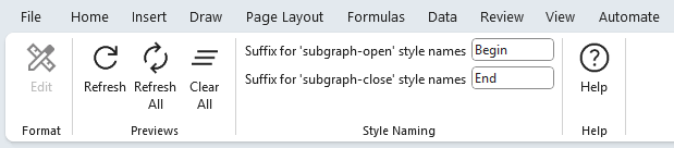
The Style Name names needed are Continent_1 Begin, Continent_2 Begin, Region_1 Begin, Region_2 Begin, with matching paired style names to close the cluster, i.e. Continent_1 End, Continent_2 End, Region_1 End, Region_2 End, with matching

Remember to include that trailing space if you are using the five pre-defined borders on the styles worksheet.

These counters are especially powerful when generating heatmaps, osage layouts, or any diagram that relies on controlled ordering or dynamic styling. By embedding {clc}, {scc}, and {rsc} directly into labels, style names, or attributes, you can assign unique visual treatments to each cluster or subcluster and enforce a predictable sort order. This makes it easy to highlight categories, create graded color schemes, or arrange elements consistently across multiple graph views.

Example 2

Use US census information to depict the 50 US states, grouping the states by by region of the country, and census division. State names should be in alphabetical order.

This is the Excel worksheet to graph:

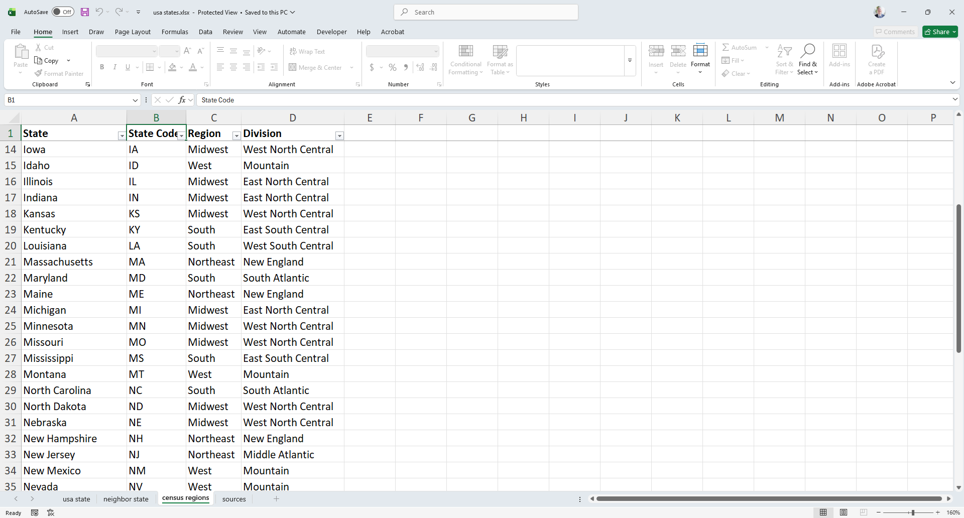
This SQL statement will process the requirements. It combines clusters, subclusters, split text and count substitution.

SELECT 
  [State Code]                      as [item],       
  'Medium Square'                   as [style name],
  'sortv={rsc}'                     as [attributes],
  [State]                           as [label],
  5                                 as [split length],
  '\l'                              as [line ending], 
  [State Code]                      as [external label],
  [State]                           as [tooltip],
  [Region]                          as [cluster],
  [Region]                          as [cluster label],
  'Border 6 '                       as [cluster style name],
  [Region]                          as [cluster tooltip],
  'sortv={clc} packmode=array_utr3' as [cluster attributes],
  [Division]                        as [subcluster],
  [Division]                        as [subcluster label],
  'Border {scc} '                   as [subcluster style name],
  [Division]                        as [subcluster tooltip],
  'sortv={scc} packmode=array_utr3' as [subcluster attributes]
FROM 
  [census regions$] 
ORDER BY 
  [Region]     ASC, 
  [Division]   ASC, 
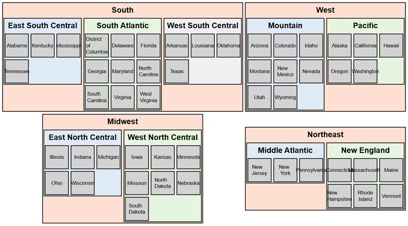
  [State Code] ASC

This is the graph produced by the data plus the SQL query.

Try it Yourself

This example is included in the samples in the Relationship Visualizer zip file in the directory 06 - Using SQL - Clusters and Subclusters.