# Using SQL

Unlock the power of SQL to extract and visualize data from your Excel spreadsheets with Relationship Visualizer. This optional feature^[1] lets you write SQL queries to pull data from multiple worksheets and generate Graphviz graphs with ease.

Ideal for users familiar with SQL, it provides a fast and flexible way to:

Combine data from multiple Excel worksheets using SQL queries
Batch‑process queries to aggregate information across several workbooks
Streamline repetitive data‑preparation and transformation tasks

SQL Topics

[1]: The SQL feature is Windows-only and requires basic SQL knowledge. If you use macOS, you can still use Relationship Visualizer’s manual data entry options.

# What is SQL?

Structured Query Language (SQL) is a domain-specific language designed for stream processing in a Relational Data Management System (RDMS). It is particularly useful in handling structured data where there are relations between different entities of the data.

SQL SELECT statements are designed to query data contained in a relational database. The SQL SELECT statement fetches data from a database, by specifying column headings, and tables from which records are to be selected, and the criteria for selection.

SELECT * is used to select all columns from a table. The FROM clause specifies the Table from which columns are to be selected. The optional WHERE clause specifies the criteria for selection.

Syntax:

    SELECT column_name FROM table_name [WHERE clause]

# Excel SQL Queries

Excel can act as a flat‑file RDBMS, accessible through ActiveX Data Objects (ADO) and SQL queries. Its SQL support is provided through a dedicated Excel‑specific dialect implemented by the Jet and ACE database engines.

TIP

See SQL Syntax for detailed information on the Excel SQL dialect.

The Relationship Visualizer includes a worksheet named sql that abstracts away most of the complexity involved in writing ADO SQL. It lets you write SQL SELECT statements using ADO‑compatible syntax, while the tool automatically manages all connection details. Queries can reference either the Relationship Visualizer workbook itself or any other Excel workbook as the data source.

When a query is executed, the results are written to the data worksheet, where they become immediately available for graphing.

ADO supports many capabilities, but the Relationship Visualizer uses only a focused subset—specifically SQL SELECT queries of the form:

SELECT [Country Code] AS [Item],
       [Country Name] AS [Label]
FROM   [Countries$]

1
2
3

This is a standard SQL query—one that selects two columns from the database (which, in this context, is an Excel worksheet) and assigns names to the results that match the column names on the data worksheet. As with a traditional database, the query specifies the name of a table; however, Excel introduces two small differences. The worksheet name must be enclosed in square brackets, and the actual sheet name—Countries in this example—must have a $ appended to it.

Square brackets are also required around column names, since Excel headers may contain spaces or special characters. Bracketing ensures ADO interprets the text as a column identifier. Quoted values cannot be used for this purpose, because quotes indicate string literals rather than column references.

# Map results to `data` worksheet columns

After the SELECT statement runs, the Relationship Visualizer processes the results and places the selected values into the corresponding columns of the data worksheet. Only recognized column names are used; all other fields are ignored. The default English column names on the data worksheet are:

[Comment]
[Item]
[Label]
[External Label]
[Tail Label]
[Head Label]
[Related Item]
[Style Name]
[Attributes]

# String constants

Excel SQL also allows you to specify string values as selection columns. When used in a SELECT statement, the string is repeated for every row returned by the query. This is particularly useful for assigning constant values such as a style name to each row of the result set.

For example, suppose the styles worksheet defines a style named Country. You can modify the query to include this style by adding a constant string column, ensuring that every row in the output is tagged with the Country style:

    SELECT [Country Code] as [Item],
           [Country Name] as [Label],
           'Country'      as [Style Name]
    FROM   [Countries$]

1
2
3
4

# Apply search conditions

SQL allows you to specify WHERE conditions to control which records are returned. The WHERE clause defines the qualifying criteria for a query. Multiple conditions can be combined using the AND and OR operators, with optional parentheses to group expressions. Only rows that meet the specified conditions are included in the results.

For example, suppose we want a list of countries that use US Dollars as their national currency. The international code for US Dollars is USD, so the SQL query would be modified as follows:

    SELECT [Country Code] as [Item],
           [Country Name] as [Label],
           'Country' as [Style Name]
    FROM   [Countries$]
    WHERE  [Currency Code] = 'USD'

1
2
3
4
5

# Eliminate duplicate values

A column often contains duplicate values. To list only the unique entries, use the SELECT DISTINCT clause. The DISTINCT keyword filters the result set so that each value appears only once, even if it occurs many times in the underlying data.

For example, if the worksheet includes a column listing the continent for each country, you can retrieve a deduplicated list of continents using a query such as:

    SELECT DISTINCT [Continent] as [Item],
           [Continent]          as [Label],
           'Continent'          as [Style Name]
    FROM   [Countries$]

1
2
3
4

# How to Use SQL in the Relationship Visualizer

Follow these simple steps to create graphs using SQL queries in Relationship Visualizer:

# Open the `sql` Worksheet

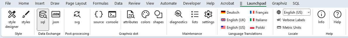
In your Relationship Visualizer workbook, use the Launchpad to show the sql worksheet, then make the sql worksheet active.

# Write Your SQL Query

Enter a SQL SELECT query using ADO syntax. For example, to create nodes for countries in the world, a simple query would look as follows:

SELECT [Country Code] as [Item],
       [Country Name] as [Label]
FROM   [Countries$]

1
2
3

Reminders:

Use square brackets [ ] for column and worksheet names.
Worksheet names end with $ (e.g., [Countries$]).

Assign column names from the data workbook to the Relationship Visualizer column names on the data worksheet. The default column names are:

[Comment]
[Item]
[Label]
[External Label]
[Tail Label]
[Head Label]
[Related Item]
[Style Name]
[Attributes]

# Specify the Excel data file

Data can be queried from any Excel workbook. Specify the workbook name in column C.

If you leave column C blank the queries will try to use a workbook specified in the Ribbon. If not present there either, it default to looking for the worksheets in the Relationship Visualizer workbook.

# Run the Query

Click the Run SQL Commands button to execute your query. The results will populate the data worksheet, with status messages in column D (e.g., SUCCESS).

# Visualize the Graph

Press the Refresh button to generate your Graphviz visualization based on the query results.

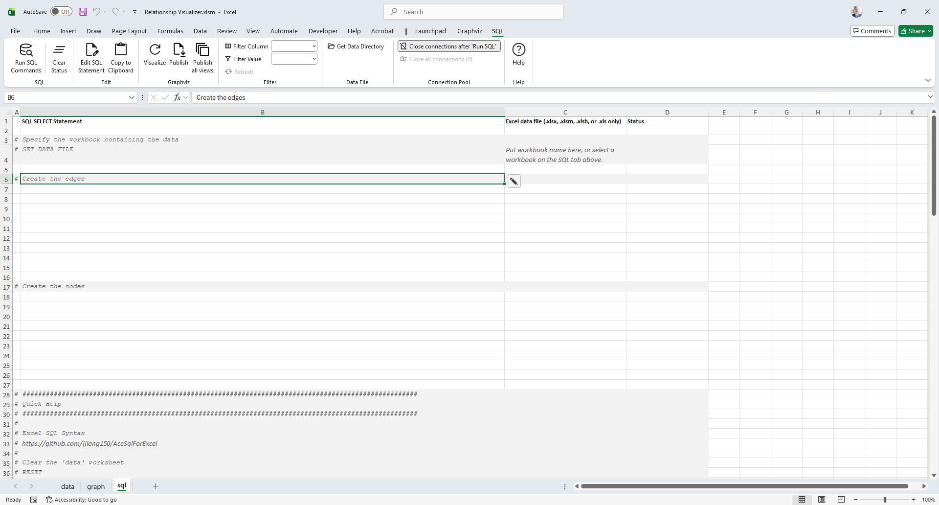
# The `SQL` Worksheet

The sql worksheet is the worksheet you will write and execute queries to pull data from another Excel workbook.

Before we run any SQL, lets gain an understanding of the mandatory and optional columns on this worksheet.

The data Worksheet has 4 columns (A-D):

A	B	C	D
Indicator	SQL SELECT Statement	Excel data file	Status

# Indicator

The Indicator column is used to draw special attention to a row.

A # hash character treats the row as a comment. The text in the row will turn gray, and this row will be skipped when running the SQL.
An ! exclamation mark character will appear if errors are detected in your data on this row. The Status will turn red, and an error message will be displayed in the Status column.

# SQL SELECT Statement

This column is where the SQL Statement is entered. For example:

SELECT [Country Code] as [Item],
       [Country Name] as [Label]
FROM   [Countries$]

1
2
3

# Excel data file

This column specifies the Excel file that contains the data.

If the column is left blank, the current Relationship Visualizer workbook is used as the data source.
If a fully qualified filename (path + file) is provided, that file is used exactly as specified.
If a relative filename (file only) is provided, it is assumed to be located in the same directory as the Relationship Visualizer workbook.

# Status

The result of the SQL query. The value will be either:

🟩 SUCCESS - The query was executed successfully.
🟥 FAILURE - The query failed. Any error message will be appended to the status value.

Even simple Excel SQL queries can fail for reasons that aren’t obvious at first glance. Keep an eye out for these common issues:
- Missing the $ in worksheet names
  ADO requires worksheet names to end with a $ (e.g., [Countries$]). Omitting it will cause the query to fail.
- 'xyz' is not a valid name. Make sure that it does not include invalid characters or punctuation and that it is not too long (where 'xyz' is a worksheet name in your FROM clause).
  
  This error usually means you have referenced a worksheet that cannot be found for one of these reasons:
  - The worksheet name is misspelled Verify that the name in your FROM clause exactly matches the worksheet tab name, including capitalization and spacing.
  - The worksheet does not exist in the Relationship Visualizer workbook. Ensure that the worksheet is present and has not been renamed or deleted.
  - No external Excel workbook was specified as a data source. ADO cannot resolve worksheet names unless a workbook has been specified.
  - The wrong Excel workbook was selected as the data source. Double‑check that the workbook you chose contains the worksheet referenced in your query.
- Forgetting square brackets around sheet or column names
  Brackets are required when names contain spaces, punctuation, or non‑alphanumeric characters.
  Examples: [Country Code], [Sales 2024$].
- Using quotes instead of brackets for identifiers
  "Country Code" is treated as a string literal, not a column reference. Always use [Country Code].
- Header row not in row 1
  ADO expects column headers in the first row of the worksheet. If your data starts lower, the query may return no rows or incorrect results.
- Mixed data types in a column
  Excel may infer the wrong type (e.g., treating numeric IDs as text). This can cause filtering or comparison operations to behave unexpectedly.
- Sheet names that look like ranges
  Names such as A1 or R1C1 can confuse the provider. Renaming the sheet usually resolves the issue.
- Hidden or filtered rows
  ADO reads the entire sheet, including hidden rows. If you expect filtered results, you must filter them in SQL.
- External workbook paths not fully pathed
  When referencing another workbook, the full path must be provided.
⬜ SKIPPED - The row was not processed because either a comment indicator (#) was present in Column A, or a Filter was applied and the row did not meet the filter criteria. Rows can be skipped for two independent reasons:
- Column A begins with #, the row is treated as a comment and is never processed.
- A Filter is active, and only rows that match the filter criteria are executed; all others are skipped.

# The `SQL` Ribbon Tab

The SQL ribbon tab is activated whenever the sql worksheet is activated. It appears as follows:

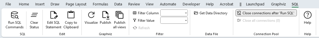
It contains the following groups, each of which is explained in the sections that follow. You may jump directly to any group using the links in this table:

Group	Controls	Description
SQL		The SQL controls let you execute the queries defined on this worksheet and manage the status information associated with each statement.

Edit		Provides tools to help get around Excel's inability to display large amounts of cell text.

Graphviz		The `sql` worksheet includes several convenience buttons designed to streamline graph generation after running SQL queries.

Filter		The Filter controls allow you to limit which rows are processed when running SQL statements.

Data File		The Data File controls let you point your SQL queries at external Excel workbooks.

Connection Pool		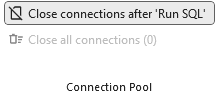The Connection Pool group manages how ADO workbook connections are reused, opened, and closed during SQL batch execution to improve performance and control file access.

Help		Provides a link to the `Help` content for the `sql` worksheet (i.e. this web page).

# SQL

The SQL controls let you execute the queries defined on this worksheet and manage the status information associated with each statement.

Label	Control Type	Description
Run SQL Commands	Button	Sequentially executes all SQL statements in the worksheet and writes the results to the `data` worksheet.
Clear Status	Button	Clears all values in the Status column, allowing you to reset or re‑run SQL statements cleanly.

# Edit

Provides tools to help get around Excel's inability to display large amounts of cell text.

Label	Control Type	Description
Edit SQL Statement	Button	Launches the Edit Text form with the contents of the currently selected cell. A second location where the Edit SQL Statement button appears is as a floating pencil button on the right side of any selected SQL cell. Clicking the pencil button performs the same action as selecting the Edit SQL Statement button in the Ribbon.
Copy to Clipboard	Button	Copies the contents of the cell as straight text to the Microsoft Windows clipboard, so it can be pasted into an external editor. Characters such as quotes are not escaped as would occur when using Excel's copy (Ctrl+C).

# Graphviz

Convenience buttons designed to streamline graph generation after running SQL queries. These controls mirror the commands on the Graphviz ribbon tab but place them closer to where SQL work is performed:

Label	Control Type	Description
Visualize	Button	Graphs the data in the `data` worksheet and displays the results in Excel. This button mirrors the Visualize command on the Graphviz ribbon tab and is provided here for faster graph creation after running SQL queries.
Publish	Button	Graphs the data in the `data` worksheet and writes the output to a file using the settings on the Graphviz ribbon tab. This duplicates the Publish command and streamlines exporting graphs after executing SQL queries.
Publish all views	Button	Graphs the data in the `data` worksheet using all defined views and writes each graph to a file based on the Graphviz ribbon settings. This matches the Graphviz ribbon's Publish all views command and accelerates batch graph generation.

# Filter

The Filter controls allow you to limit which rows are processed when running SQL statements. This is especially useful when working with large datasets or when you want to preview results for a specific subset of data.

Label	Control Type	Description
Filter Column	Dropdown list	Lists column letters E–Z. Select the column you want to filter on.
Filter Value	Dropdown list	Displays all unique (de‑duplicated) values found in the selected Filter Column. When a value is chosen, SQL statements will run only on rows where that column matches the selected value.
Refresh	Button	Updates the Filter Value list. Use this after changing data in the selected Filter Column to ensure the dropdown reflects the latest values.

# Data File

The Data File controls let you point your SQL queries at external Excel workbooks. This is especially useful when your data is stored in multiple files—such as monthly extracts, departmental exports, or versioned snapshots—and you want to run the same SQL queries against each file without rewriting anything.

Label	Control Type	Description
Get Data Directory	Button	Opens a directory‑picker dialog. When a folder is selected, its path replaces the “Get Data Directory” label.
File Name	Dropdown list	Lists the Excel files found in the selected directory that are suitable for running Excel SQL queries against. This list is only visible when a data directory has been specified. NOTE: Entries in the file name column, and `SET DATA FILE` statements take precedence when resolving conflicts over which data source to use.
Reset	Button	Clears the data directory and file name selections. This button is only visible when selections have been made

Why would I use this?
Many workflows produce recurring Excel extracts—for example, one workbook per month, quarter, or reporting cycle. By selecting a directory and choosing a file from the dropdown, you can run the same SQL queries against each extract in turn. This makes it easy to compare periods, regenerate graphs for new data, or batch‑process multiple datasets without modifying your SQL.

# Connection Pool

The Connection Pool group manages how ADO workbook connections are reused, opened, and closed during SQL batch execution to improve performance and control file access.

Connection pooling was added in Version 7.0 in response to a March 2025 Office update that caused ADO connections to take over 12 seconds (previously under 4 milliseconds). See: Excel ADO connection issue in recent Office 365 update (opens new window)

Workbook connections are now reused across all SQL statements during a Run SQL Statements batch run.

Users can choose to close connections after batch execution or keep them open until manually closed or until the workbook exits.

Note: Keeping connections open may improve performance but can prevent access to referenced workbooks.

Label	Control Type	Description
Close connections after 'Run SQL'	Toggle Button	Determines whether connections remain open (pooled) after running SQL statements or are closed immediately after execution.
Close all connections (#)	Button	Displays the number of currently open connections. Enabled only when one or more connections are open. Pressing the button closes all open connections.

When should I keep connections open?

Keeping connections open (pooled) is most beneficial when running many SQL statements in a batch, especially if each statement targets external workbooks. Reusing the same connection avoids repeated ADO initialization overhead and can dramatically improve performance.

However, if you need to open, edit, or replace any referenced workbooks, you may prefer to close connections after each run to avoid file‑locking issues.

# Help

Provides a link to the Help content for the sql worksheet (i.e. this web page).

Label	Control Type	Description
Help	Button	Provides a link to this web page.

# The `Edit SQL Statement` Form

Excel rows can hold a great deal of information, but cells have their quirks. Each cell can store up to 32,767 characters, yet only about 1,024 of them are visible directly in the grid without entering cell‑edit mode. For rows, the practical display limit depends on the combined content of each cell, though in reality screen size and readability become limiting factors long before Excel’s technical limits are reached. These limits get reached quickly if you like to break SQL statements down over multiple lines. In short, you can store a lot—but you may not be able to see it all at once.

To address this, Version 7 introduced an Edit SQL Statement form. When you press the Edit SQL Statement button, a modal window opens containing the full text of the currently selected cell, making it easier to view and edit long content without fighting Excel’s display constraints.

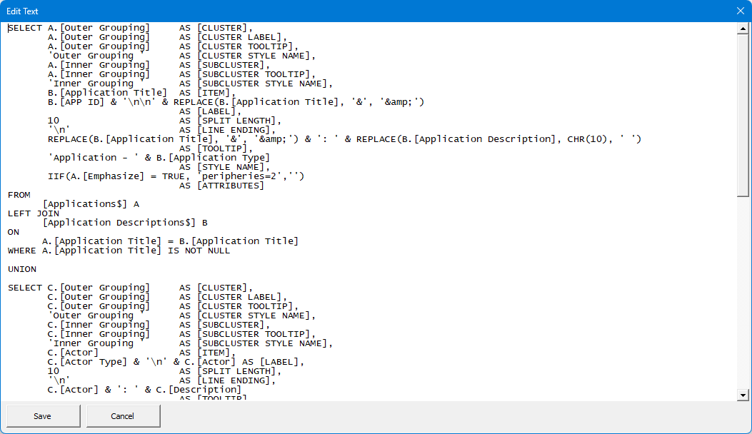
Horizontal and vertical scroll bars are provided to help navigate the text. You can change the text within the form.

Pressing the Save button transfers the contents from the form back to the active cell.

# Next Steps

The topics above introduce the core ways to use SQL within Relationship Visualizer. For more detailed, step‑by‑step lessons and reference material, explore the following pages:

Like this tool? Buy me a coffee! ☕ (opens new window)

← Styles SQL Queries for Creating Graphs →

# Using SQL

# What is SQL?

# Excel SQL Queries

# Map results to data worksheet columns

# String constants

# Apply search conditions

# Eliminate duplicate values

# How to Use SQL in the Relationship Visualizer

# Open the sql Worksheet

# Write Your SQL Query

# Specify the Excel data file

# Run the Query

# Visualize the Graph

# The SQL Worksheet

# Indicator

# SQL SELECT Statement

# Excel data file

# Status

# The SQL Ribbon Tab

# SQL

# Edit

# Graphviz

# Filter

# Data File

# Connection Pool

# Help

# The Edit SQL Statement Form

# Next Steps

# Map results to `data` worksheet columns

# Open the `sql` Worksheet

# The `SQL` Worksheet

# The `SQL` Ribbon Tab

# The `Edit SQL Statement` Form